Algorithms sensitivity to single salient dimension

Posted on Fri 23 January 2015 in Notebooks

Sensitivity to 1 salient dimension

How different classifiers managers to sort through noise in multidimensional data

In this experiment I will test different machine learning algorithms sensitivity to data where only 1 dimension is salient and the rest are pure noise. The experiment tests variations of saliency against a number of dimensions of random noise to see which algorithms are good at sorting out noise.
For experiments performed here, there will be a 1-1 mapping between the target class in $y$ and the value of the first dimension in a datapoint in $x$. For example, for all datapoints belonging to class 1, the first dimension will have the value 1, while if the datapoint belongs to class 0, the first dimension will have the value 0.

In [10]:
#Configure matplotlib
import matplotlib.pyplot as plt
from mpl_toolkits.mplot3d import Axes3D
%pylab

#comment out this line to produce plots in a seperate window
%matplotlib inline 
figsize(14,5)
Using matplotlib backend: MacOSX
Populating the interactive namespace from numpy and matplotlib

Data

First the target vectors $y$ and $y_4$ are randomly populated. $y\in[0,1]$ and $y_4\in[0,1,2,3]$. The for each value in $y$ and $y_4$ a datapoint is generated consisting of the value of the target class, followed by 100 random values. This way the first column in the data matrix is equal to the target vector. Later this column will be manipulated linearly.

In [11]:
#initialize data

def generate_data():
    ''' Populates data matrices and target vectors with data and release it into the global namespace 
        running this function will reset the values of x, y, x4, y4 and r '''
    global x, y, x4, y4, r
    y = np.random.randint(2, size=300)
    y4 = np.random.randint(4, size=300)
    r = np.random.rand(100, 300)
    x = np.vstack((y,r)).T
    x4 = np.vstack((y4,r*4)).T

generate_data()

# note that x and y are global variables. If you manipulate them, the latest manipulation of x and y will
# used to generate plots.
    
split = 200
max_dim = x.shape[1]
m = 1
y_cor = range(m, max_dim)

print 'y is equal to 1st column of x:  \t', list(y) == list(x[:,0])
print 'y4 is equal to 1st column of x4:\t', list(y4) == list(x4[:,0])
print '\nChecking that none of the randomized data match the class values
print 'min:\t', r.min(), 'max:\t',r.max(), '\tThese should never be [0,1], if so please rerun.'
y is equal to 1st column of x:  	True
y4 is equal to 1st column of x4:	True
min:	5.75157395193e-05 max:	0.999952558364 	These should never be [0,1]

Visualizing the data

This section will plot parts of the data to give the reader a better understanding of its shape.

In [12]:
plt.subplot(121)
plt.title('First 2 dimensions of dataset')
plt.plot(x[np.where(y==0)][:,1],x[np.where(y==0)][:,0], 'o', label='Class 0')
plt.plot(x[np.where(y==1)][:,1],x[np.where(y==1)][:,0], 'o', label='Class 1')
plt.ylim(-0.1, 1.1) #expand y-axis for better viewing
legend(loc=5)

plt.subplot(122, projection='3d')
plt.title('First 3 dimensions of dataset')
plt.plot(x[np.where(y==0)][:,2],x[np.where(y==0)][:,1],x[np.where(y==0)][:,0], 'o', label='Class 0')
plt.plot(x[np.where(y==1)][:,2],x[np.where(y==1)][:,1],x[np.where(y==1)][:,0], 'o', label='Class 1')
Out[12]:

A clear seperation between classes is revealed when visualized. This clear seperation between the 2 classes remains, no matter how many noisy dimensions we add to the dataset, so in theory it is reasonable to expect any linear classifier to find a line that seperates the 2 datasets.

In [13]:
#Initialize classifiers

from sklearn.neighbors import KNeighborsClassifier as NN
from sklearn.svm import SVC as SVM
from sklearn.naive_bayes import MultinomialNB as NB
from sklearn.lda import LDA
from sklearn.tree import DecisionTreeClassifier as DT
from sklearn.ensemble import RandomForestClassifier as RF
from sklearn.linear_model import Perceptron as PT

classifiers = [NN(),NN(n_neighbors=2), SVM(), NB(), DT(), RF(), PT()]
titles = ['NN, k=4', 'NN, k=2', 'SVM', 'Naive B', 'D-Tree', 'R-forest', 'Perceptron']

# uncomment the following to add LDA
#classifiers = [NN(),NN(n_neighbors=2), SVM(), NB(), DT(), RF(), PT(), LDA()]
#titles = ['NN, k=4', 'NN, k=2', 'SVM', 'Naive B', 'Perceptron', 'LDA']
#m, y_cor= 2, range(m, max_dim)
In [14]:
# define functions
def run (x,y):
    '''Runs the main experiment. Test each classifier against varying dimensional sizes of a given dataset'''
    
    global score
    score = []
    for i, clf in enumerate(classifiers):
        score.append([])
        for j in range(m,max_dim):
            clf.fit(x[:split,:j],y[:split])
            score[i].append(clf.score(x[split:,:j], y[split:]))

def do_plot():
    ''' Generates the basic plot of results 
        Note:   Score is a global variable. The latest score calculated from run()
                will always be used to draw a plot '''
    
    for i, label in enumerate(titles):
        plt.plot(y_cor, score[i], label=label)
    plt.ylim(0,1.1)
    plt.ylabel('Accuracy')
    plt.xlabel('Number of dimensions')

def double_plot():
    ''' Runs the experiment for 2 classes and 4 classes and draws appropriate plots 
        Note:   x and y are global variables. The latest manipulation of these are
                always used to run the experiment. If you need 'original' x and y's
                you need to rerun generate_data() and use new randomized data '''
    
    plt.subplot(121)
    plt.title('Two classes')
    run(x,y)
    do_plot()
    plot([0,100], [0.5,0.5], 'k--') #add baseline
    plt.legend(loc=3)
    plt.subplot(122)
    plt.title('Four classes')
    run(x4,y4)
    do_plot()
    plot([0,100], [0.25,0.25], 'k--') #add baseline

Experiment 1

Test all classifiers against 2 class and 4 class datasets for 1 through 100 dimensions. Notice that Naive Base fails when the dataset is literally equal to the targets, but adding just a little bit of noise and it starts to work much better.

For 4 classes, Naive Base again starts of poorly, but while the other algorithms quickly succumb to the noisy dimensions, Naive Bayes seems to improve up until ~20 dimension, and though its performs starts to decline, it is still the best performer from there on out. If you are running the experiment with LDA, then the test will not be done for 1 dimension, and Naive Bayes weakest point won't show.

However, the Decision Tree is quick to find that one dimension explains everything, and has no trouble throughout either experiment. The random forest have some trees where the salient dimension has been cut off, so more noise and randomness is added to the results.

In [15]:
double_plot()

Experiment 2

In this experiment the first column of the data matrix is linearly manipulated in order to "hide" the values that map to the classes better amongst the noise. For 2 classes experiment the value 0.25 maps to class 0 and 0.75 maps to class 1. For the 4 class experiment, value:class mapping is now 1:0, 1.5:1, 2:2, 2.5:3, 3:4 This does not change the fact that there is a clear boundry between the classes. It just means the distance between the 2 planes seen in the visualization section is getting narrower.

In [16]:
plt.figure()
x[:,0] = (x[:,0]/2)+0.25
x4[:,0] = (x4[:,0]/2)+1

double_plot()

This experiment is quite sensitive to the randomness in the data. For two classes in general the SVM is the strongest until around the 40 dimension mark, where the Naive Bayes takes over. In the higher dimension area, NN often manages to overtake SVM, though this is somewhat dependent on the random data. It's still surprising, given that NN is usually the poster child for the curse of dimensionality. It is not that easy to hide linear explanation for to the Decision Tree, which clearly outperforms everything here. The tendency to overfitting is really helping.

Baseline test (random only)

In this final experiment the only salient datapoint in the observation data is removed to show the reader that this will attain baseline results. Also notice, depending on the data, the baseline for some of the algorithms can be as high as 60% accuracy. Keep this in mind when reviewing results from above.

In [17]:
x = x[:,1:]
x4 = x4[:,1:]

double_plot()
plt.legend(loc=1)
plt.subplot(121)
plt.legend().remove()

Some notes on unicode and UTF-8 and its various representations

Posted on Thu 13 November 2014 in Notes

When working with NLP on a wide variety of text, one is bound to encounter various encoding trouble. Even when everything is revolving around unicode, things are not as straightforward as one could hope.

Here's an example of some trouble with a series of files named by a string representation of the hexadecimal value of the utf-8 unicode codepoint.

File names:

  • E6B7B1.png
  • E6B48B.png
  • E6B88B.png
  • ...

In my case they look something like this:

Stroke order diagram for 母

Stroke order diagram converted to png from the KanjiVG project

The problem is to convert these back into unicode, so it is possible for a human to read what the names actually represent. This is easy to do, but difficult to learn how to.

The file names are UTF-8 hex, not unicode codepoints. The Absolute Minimum Every Software Developer Absolutely, Positively Must Know About Unicode and Character Sets (No Excuses!) guide has a nice explanation of what is going on here, the important part being this (emphasis mine):

Thus was invented the brilliant concept of UTF-8. UTF-8 was another system for storing your string of Unicode code points, those magic U+ numbers, in memory using 8 bit bytes. In UTF-8, every code point from 0-127 is stored in a single byte. Only code points 128 and above are stored using 2, 3, in fact, up to 6 bytes.

So what we are seeing are 3 bytes encoded in hexadecimal that refers to some unicode codepoint (which again refers to an actual character)

In python we can use the string.decode() function to handle these 2 conversions. First we convert the ascii hex representations into actual hex and then we convert the hex numbers into the unicode codepoint that they refer to.

>>>> 'E6B88B'.decode('hex').decode('utf-8')
u'\u6e0b'
>>> print(u'\u6e0b')
渋

My full script is as follows

The python script:

# -*- coding: utf-8 -*-
"""
@author: Mads Olsgaard, 2014

Released under BSD3 License.

This scripts renames .png files that are named with hexadecimal values into their utf-8 string. Assumes the form of A1E2B3.png

Thanks to user plaes @ http://stackoverflow.com/a/13358677
"""

import glob, os, shutil

basepath = '../path_to/hex2utf/' #folder where we want to take our files from
targetpath = basepath+'out/' # path to where we want to store the renamed files

pattern = '??????.png'     # pattern of the file name. In this case we are only looking for 6 character long file names of the png type.
                        # These are not regex. See https://docs.python.org/3/library/fnmatch.html

filelist = glob.glob(basepath+pattern) #load all files in basepath that conform to pattern

# Extract the filename from each file path in filelist, truncate the '.png' section
# The .decode('hex').decode('utf-8') part is where the magic happens. First we convert the ASCII string into the hex values it represents
# 'E6B88B' -> '\xe6\xb8\x8b'
# and then we convert the hex-code into the UTF8 unicode character that it represents
# '\xe6\xb8\x8b' -> u'\u6e0b', which in unicode aware applications will show up as '渋'

filenames = [os.path.basename(n)[:-4].decode('hex').decode('utf-8') for n in filelist]

for n,t in zip(filelist, filenames):
    shutil.copy2(n, targetpath+t+'.png')

Some other links worth looking at


Basics of Kana-kanji conversion

Posted on Tue 04 November 2014 in Notes

A kana/kanji conversion system goal is to convert a string of phonetical characters – kana – into a string of mixed logographic kanji and phonetic kana. That is, we want to go from ごはんをたべます →ご飯を食べます (To eat a meal).

Let $W$ be a set of words ${w_1, w_2 ... w_n}$ in a sentence (in the above example W would be ご飯を食べます). $P(W)$ is the probability that this sentence exists in the language. In practice that is, how many times does this exact sentence show up in our training data. Since very few sentences show up in written language more than once, the chance that we will deal with a sentence that does not exist in our training set is quite high. Therefore we tend to let $W$ be a collection of uni, bi, and trigrams and their associated frequenzy. $P(W)$ is also known as our language model.

Let $A$ be a string of phonetic characters – or kana – so that $A = {a_1, a_2 ... a_m}$.

Now we want to find the most probable string $W$ associated with the input string $A$.

A classic example is きしゃのきしゃがきしゃのきしゃできしゃした which we typically want to Picture of mounted archery "きしゃ"be 貴社の記者が貴社の汽車で帰社した (Your reporter was sent home in your train). Given that all the nouns in the phrase is pronounced きしゃ(kisha) this leads to a large variety of more or less meaningful, but still possible sentences. The reporter could be sent home in the reporters own train, or the train could be sent home on the reporter. The reporter or train could even be involved in mounted archery (騎射 also read きしゃ) if one is imaginative enough. However entertaining that may be, it is the job of our kana-kanji converter to convert to the most likely sentence, not the most entertaining.

Using Bayes theorem we can ask What is the probability of an observed kana string A, given a sentence W?

$$P(W|A) = \frac{P(A|W)P(W)}{P(A)} $$

[1]

And we want to find the W that maximizes this probability, so that $W^* = arg_wmaxP(W|A) =  arg_wmax\frac{P(A|W)P(W)}{P(A)}$

We tend to assume that users will correctly type the kana input that they intend to type. That is, there are no typos and there are no spelling mistakes (note the general absence of Japanese spellcheckers in the market place). So we can assume that $P(A) = 1$.

We can make a few more assumptions about the Japanese language. For example, if we have a sentence W, then we can be very certain that there is only 1 kana string A that fits. ご飯を食べます can only be read ごはんをたべます in basically any circumstance that we would come across. So $P(A|W)=1$, for most sentence and we can further reduce [1] to $$P(W|A) = P(W) $$ or to put it in a different way, the most likely correct sentence is completely dependent on the language model ((Suzuki, Hisami, and Jianfeng Gao. Microsoft Research IME Corpus. Microsoft Research Technical Report, 2005. http://131.107.65.14/pubs/70243/tr-2005-168.pdf.

)).

Caveats

However, things are not always as simple as described above.

Input string A and P(A)

We assume input to be a string of phonetic character representations that we must convert into an actual sentence, very much like how we would do in a text-speech system. However, to complicate matters, both input and output strings will often contain alphanumeric characters as well as punctuation. Some of these – such as numbers – may have an effect on how conversion of following kana must be done, others characters – mostly alphabet characters – will not and it might be best to ignore such characters during conversion, especially if we suspect the user to input very creative emoticon that we haven't met in the training data. However, we may want to substitute single width alphabet to double width and we may or may not want to convert alphabet into kana.

Moreover, we assume the user to type correctly. There appears to be very little research into what kind of spelling mistakes Japanese writers tend to make when typing Japanese on a keyboard or smartphone. There exist research on the errors people make when writing by hand or when typing English, but it appears to be silently assumed by academics that Japanese authors type correctly. It does seem unlikely, though, that Japanese writers never forget to add a ” or make a や or a ゆ small. A literature search only found 1 paper dealing with proofing written Japanese ((Takeda, Koichi, Emiko Suzuki, Tetsuro Nishino, and Tetsunosuke Fujisaki. “CRITAC—An Experimental System for Japanese Text Proofreading.” IBM Journal of Research and Development 32, no. 2 (1988): 201–16.

)), while more research appears to have gone into how Japanese writers misspell English text ((Ishikawa, Masahiko. Apparatus for Correcting Misspelling and Incorrect Usage of Word. Google Patents, 1998. http://www.google.com/patents/US5812863.

Mitton, Roger, and Takeshi Okada. “The Adaptation of an English Spellchecker for Japanese Writers,” 2007. http://eprints.bbk.ac.uk/592.

)).

**

So in the real world, $P(A) \ne 1$**

Unambiguity of the reading of a known sentence

Earlier I described how we can assume $P(A|W) = 1$. This is an important assumption for a lot of practical reasons. Mainly, because training data is expensive to annotate, but with this assumption we can annotate training data with kana readings automatically, without human intervention. This is how Baidu ((Wu, Xianchao, Rixin Xiao, and Xiaoxin Chen. “Using the Web to Train a Mobile Device Oriented Japanese Input Method Editor,” 2013. http://www.aclweb.org/anthology/I/I13/I13-1172.pdf.

)) is able to build a 2.5 terabyte training corpus from the web. This would be impossible to annotate by hand.

But the readings of a Japanese sentence is ambiguous at times. 今日 can in basically every instance it occurs in Japanese be read either きょう or こんにち, with the latter being too polite for most occasions, but still a possibility. If we expand the earlier example sentence to 私はご飯を食べます (I eat a  meal) it is impossible to deduce if the author meant to use the very polite わたくし or the normal わたし. Given that most automated will convert 私 into わたし we get a self reenforcing that the shorter form should be used.

So in the real world, $P(A|W) \ne 1$


Bell curves, normal distributions and Gaussians

Posted on Mon 27 October 2014 in Notes

While it is much better to refer to such a curve as a ‘normal distribution' than as a ‘bell curve,' if you really want to fit into the Statistical NLP or pattern recognition communities, you should instead learn to refer to these functions as Gaussians, and to remark things like, ‘Maybe we could model that using 3 Gaussians' at appropriate moments.'

– Foundations of Statistical Natural Language Processing


Showing Japanese characters in Matplotlib on Ubuntu

Posted on Mon 27 October 2014 in Notes

TL;DR: Install Japanese language support and insert the following in your python script

import matplotlib
matplotlib.rc('font', family='TakaoPGothic')

If you are working with any kind of NLP in Python that involves Japanese, it is paramount to be able to view summary statics in the form of graphs that in one way or another includes Japanese characters.

Below is a graph showing Zipf's Law for the distribution of characters used in [TL;DR: Install Japanese language support and insert the following in your python script

import matplotlib
matplotlib.rc('font', family='TakaoPGothic')

If you are working with any kind of NLP in Python that involves Japanese, it is paramount to be able to view summary statics in the form of graphs that in one way or another includes Japanese characters.

Below is a graph showing Zipf's Law for the distribution of characters used in](http://en.wikipedia.org/wiki/Tetsuko_Kuroyanagi) ‘Totto Channel', the sequel to her famous “Totto Chan: The little girl by the window”.


Character Distribution of 100 most used characters - but which ones?

Character Distribution of 100 most used characters - but which ones?


On most systems, Matplotlib will not be able to display Japanese characters out-of-the-box and this is a big problem as the graph above is completely useless for even the most basic investigation.

I've tested on OSX, Windows 8 and Ubuntu and only OSX manages to work out of the box, despite my Windows installation being Japanese!

Most advice online will tell you to change the font used by Matplotlib, but if you are on Ubuntu it might not be completely obvious which font you need to use! Moreover there are many ways to change the font.

I've found the simplest way of changing fonts to simply be using matplotlib.rc

import matplotlib
matplotlib.rc('font', family='Monospace')

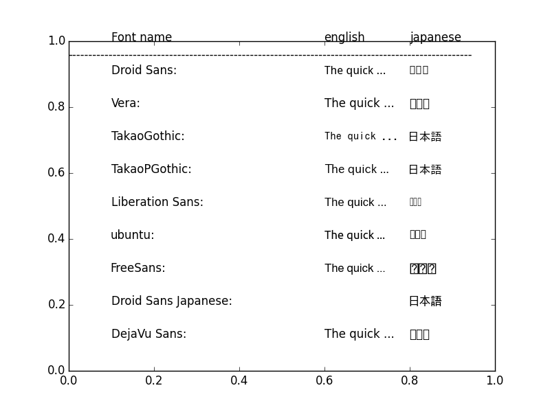
In family you can either insert the name of a font family (as in the above example) or you can name a specific font, which is what you want to do in this case. But which one? I wrote the following script to help check which fonts will work.

# -*- coding: utf-8 -*-
"""
Matplotlib font checker
Prints a figure displaying a variety of system fonts and their ability to produce Japanese text

@author: Mads Olsgaard, 2014

Released under BSD License.
"""

import matplotlib
import matplotlib.pyplot as plt
from matplotlib import font_manager

fonts = ['Droid Sans', 'Vera', 'TakaoGothic', 'TakaoPGothic', 'Liberation Sans', 'ubuntu', 'FreeSans', 'Droid Sans Japanese', 'DejaVu Sans']
#fonts = ['Arial', 'Times New Roman', 'Helvetica'] #uncomment this line on Windows and see if it helps!
english = 'The quick ...'
japanese = '日本語'
x = 0.1
y = 1

# Buils headline
plt.text(x+0.5,y, 'english')
plt.text(x+0.7, y, 'japanese')
plt.text(x,y, 'Font name')
plt.text(0,y-0.05, '-'*100)
y -=0.1

for f in fonts:
    matplotlib.rc('font', family='DejaVu Sans')
    plt.text(x,y, f+':')
    matplotlib.rc('font', family=f)
    plt.text(x+0.5,y, english)
    plt.text(x+0.7, y, japanese)
    y -= 0.1
    print(f, font_manager.findfont(f))  # Sanity check. Prints the location of the font. If the font it not found, an error message is printed and the location of the fallback font is shown

plt.show()

On ubuntu the output should be the following:

Droid Sans /usr/share/fonts/truetype/droid/DroidSans.ttf
Vera /home/supermads/anaconda3/lib/python3.4/site-packages/matplotlib/mpl-data/fonts/ttf/Vera.ttf
TakaoGothic /usr/share/fonts/truetype/takao-gothic/TakaoGothic.ttf
TakaoPGothic /usr/share/fonts/truetype/takao-gothic/TakaoPGothic.ttf
Liberation Sans /usr/share/fonts/truetype/liberation/LiberationSans-Regular.ttf
ubuntu /usr/share/fonts/truetype/ubuntu-font-family/Ubuntu-R.ttf
FreeSans /usr/share/fonts/truetype/freefont/FreeSans.ttf
Droid Sans Japanese /usr/share/fonts/truetype/droid/DroidSansJapanese.ttf
DejaVu Sans /usr/share/fonts/truetype/dejavu/DejaVuSans.ttf

As you can see, I'm running Anaconda Python 3, and if Anaconda can't find a font it will fallback into it's own folder to load the Vera font.

Font check

Surprisingly, Droid does support Japanese, it just saves the Japanese character space in a seperate font file, rendering it useless for this purpose. However, the Takao font family does work for our purpose.

Takao fonts should be installed by default if you have set your location somewhere in Japan during installation of Ubuntu or if you have installed support for Japanese language in System SettingsLanguage Support (just hit the super key and search for language). I recommend this, since this will also install the Japanese input method, Anthy

You can also use apt-get, like this from the command line (not tested):

sudo apt-get install fonts-takao-mincho fonts-takao-gothic fonts-takao-pgothic

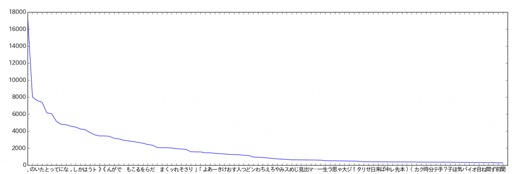
And now we can finally see which characters Kuronayagi used the most for her sequel:

Character Distribution of 100 most used characters

And apparently, that's the Japanese comma, also called 読点